It is about my endeavors to create some neat plots of the results obtained using the proprietary DFT program VASP one and a half years ago. Since these files are usually pretty big it is important for your plotting script to rely on compiled C, C++ or Fortran code under the hood of a high level language like R or python. And you definitely want to have one of the latter ones for creating you plots since it is way more easy and beautiful.
I wrote a couple of functions handling both the import and the manipulation of the CHGCAR and CHG files of VASP’s output including C++ functions speeding them up. So it felt quite naturally to pack them all together and make them available for other users. But as a disclaimer: I haven’t worked with VASP in years and neither do I intend to do it anymore nor have I access to the program. But anyway I will of course try my best to support you in case of questions or bugs in the vasp2R package.
Data
This vignette shows the basic usage of the vasp2R package. First we will import an example CHG file, do some manipulation and finally plot the result of the VASP calculation.
The VASP files used to create the CHG file supplied by this package are taken from the third Hands-on example of VASP’s documentation. I used the first one: the clean Ni surface. Why did I used the CHG and not the CHGCAR? Because it also contains the required information but is smaller in size and I want to keep package’s size at a minimum.
Import
First of all you have to be sure of have the vasp2R package installed.
check.validity <- try( library( "vasp2R" ), silent = TRUE )
if ( class( check.validity ) == "try-error" ){
    ## the package is not installed yet
    devtools::install_github( "theGreatWhiteShark/vasp2R" )
    library( vasp2R )
}
During installation the CHG files is copied as one of the package’s assets on the hard disk. We will import it into R using the vasp.import function.
data.imported <- vasp.import( system.file( "example/CHG",
                                          package = "vasp2R" ) )
Structure of the imported vasp object
The resulting object data.imported is of class vasp and inherits from the list class. It has three named elements: charge, atoms, and lattice.
charge
The charge element represents the charge density in the three dimensional unit cell. It itself is of class data.frame and contains four named columns: x, y, z, charge.
atoms
The atoms element represents the coordinates and the type of the individual atoms in the unit cell. It is derived from the CONTCAR like entry in the CHGCAR/CHG file. So the type value corresponds to the VASP internal string representation of the periodic table (e.g. “Si” for silicon). It is of class data.frame and consists of four named columns: x, y, z and type
lattice
The lattice element is a data.frame representing the lattice vectors of the unit cell. It contains three named columns: x, y and z and the entries of a specific row correspond to a specific vector.
Manipulation of the vasp object
Reproducing the unit cell
Afterwards we will reproduce the imported VASP results of a single Ni atom with periodic boundary conditions to make it actually look like a surface.
data.reproduced <- vasp.reproduce( data.imported, x.rep = seq( -3, 3 ),
                                  y.rep = seq( -3, 3 ) )
## the x.rep, y.rep and z.rep argument of the vasp.reproduce function
## have to be supplied using a numerical vector. In the above example
## the unit cell is going to be reproduced three times in the positive
## and negative direction along both the x and y axis.
Most of the functions in vasp2R can be called with either the whole object of class vasp or with the individual elements. So its also possible to call vasp.reproduce( data.imported$atoms ) to calculate just a reproduced version of the atomic positions.
Rotating the surface
We can also rotate the positions to change our point of view. For such a clean and symmetric surface this is a little bit useless. But for more complex structures it will become quite handy.
data.rotated <- vasp.rotate.cell( data.reproduced, angle = 45* pi/ 180 )Creating bonds between atoms
Then we establish bonds between the individual atoms (for a better visualization of the results).
data.bonds <- vasp.bonds( data.rotated, distance = 8 )The vasp.bonds function will create bonds between all atoms closer together than the supplied distance value within the x-y plane.
Further modifications
Another function implemented in vasp2R is vasp.diff. It expects two objects of class vasp as input and creates a new one of the same type containing the charge differences of the first input minus the second one. It also holds all the atoms and lattice entries of the first argument and is therefore a fully fledged vasp object.
Visualization
In principle you can use whatever plotting package you want. But personally I would recommend the usage of the ggplot2 package.
But before we start visualizing anything, how do we plot the charge density? My approach is to slice the three dimensional charge density in individual planes and plot those along with the atoms in the plane.
There are two main problems in visualizing the charge density:
- The spacing of the charge density values provided by the CHGCAR is not compatible with the one the ggplot2 libraries accept. This actually leads to a huge number of tiny rectangle getting plotted and you won’t even be able to see. That’s how tiny they gonna be.
- There are way to much charge density values. If one intends to save the plot as a vector graphic you would end up with several GB even for moderate sized unit cells (simply because they contain hundreds of thousand points)
So instead we create an evenly grid of variable size and calculate the mean charge density in each of those grid boxes.
library( ggplot2 )
library( RColorBrewer ) # For nice colors out of the bxo
color.atom <- "navy"
color.gradient <- "YlOrRd" # a RColorBrewer palette

## Here we will create a plot function taking a z value, create
## a slice at this specific value and plots it along with the atomic
## positions in the x-y plane
vasp.plot <- function( vasp.input, z = 0, grid.point.number = 20 ){
    ## Check out RColorBrewer::brewer.pal.info for different ones

    ## Determine the z grid point closed to the supplied z value
    ## This is not the actual height value but its index in
    ## vasp.input$charge$z!
    plot.height <- which( abs( unique( vasp.input$charge$z ) - z ) ==
                          min( abs( unique( vasp.input$charge$z ) - z ) ) )
    ## Extract just those values of the charge density corresponding to
    ## the determined slice grid point
    slice.charge <-  vasp.input$charge[
        vasp.input$charge[ "z" ] == unique( vasp.input$charge$z )[
                                              plot.height ], ]
    ## Same for the atoms
    plot.atoms <-  vasp.input$atoms[
        vasp.input$atoms[ "z" ] == unique( vasp.input$atoms$z )[
                                             plot.height ], ]

    ## Constructing a grid for plotting the charge density
    ## Boundaries of the charge density
    limits.x <- c( min( slice.charge$x ), max( slice.charge$x ) )
    limits.y <- c( min( slice.charge$y ), max( slice.charge$y ) )

    ## Creating the grid
    plot.charge <- expand.grid( x = seq( limits.x[ 1 ],
                                          limits.x[ 2 ], ,
                                          grid.point.number ),
                                 y = seq( limits.y[ 1 ],
                                         limits.y[ 2 ], ,
                                         grid.point.number ) )

    ## Width of the grid boxes
    grid.width.x <- unique( plot.charge$x )[ 2 ] -
                      unique( plot.charge$x )[ 1 ]
    grid.width.y <- unique( plot.charge$y )[ 2 ] -
                      unique( plot.charge$y )[ 1 ]

    ## Calculate the mean charge density for all points within one grid
    ## box
    plot.charge$charge <- Reduce( c, apply( plot.charge, 1, function( row ){
        charge <- mean( slice.charge$charge[
            abs( slice.charge$x - as.numeric( row[ 1 ] ) ) <=
                grid.width.x &
            abs( slice.charge$y - as.numeric( row[ 2 ] ) ) <=
                grid.width.y ] )
        return( charge )
    } ) )

    ## the actual plotting
    ggplot() +
        ## Plotting the charge density of the slice
        geom_raster( data = plot.charge, interpolate = TRUE,
                  aes( x = x, y = y, fill = charge ) ) +
        ## Plotting the atoms
        geom_point( data = plot.atoms, color = color.atom, stroke = 1.5,
                   aes( x = x, y = y ), shape = 16, size = 4 ) +
        ## Customized the color scale of the charge density
        scale_fill_distiller( palette = color.gradient, direction = 1 ) +
        ## Remove the grid lines in the ggplot plot
        theme_bw() +
        theme( panel.grid.major = element_blank(),
              panel.grid.minor = element_blank(),
              panel.background = element_blank() )

    ## Via this functions additional elements can be introduced to the
    ## plot after calling this function
    return( last_plot() )
}

vasp.plot( data.imported, 0, 20 )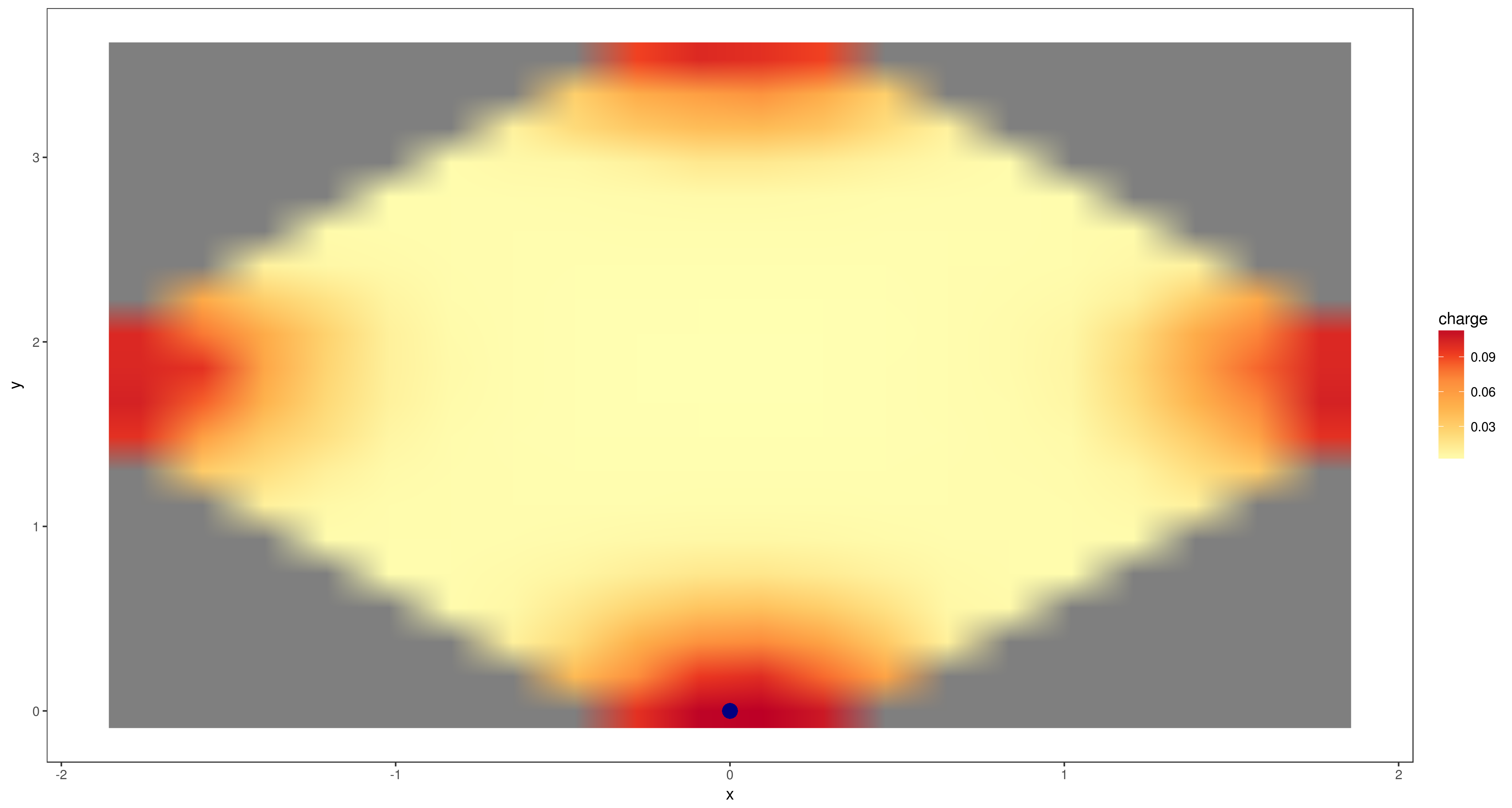
And for the reproduced one
vasp.plot( data.reproduced, 0, 20 )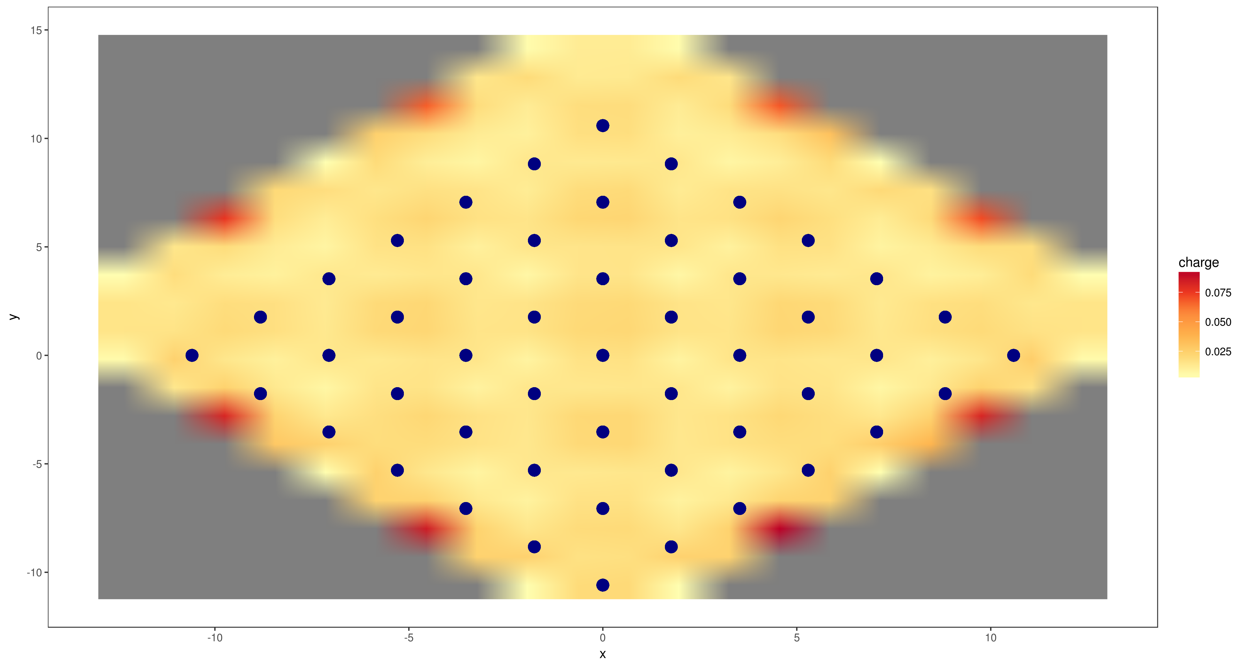
Pretty good so far. Now lets introduce the bonds to the plotting.
The data.bonds$bonds element contains the point of the beginning and end of all the extracted bonds.
vasp.plot( data.bonds, 0, 20 ) +
    ## extract just the bonds within the considered plane
    geom_segment( data = data.bonds$bonds[
                      data.bonds$bonds$z.begin == 0 &
                      data.bonds$bonds$z.end == 0, ],
                 aes( x = x.begin, y = y.begin, xend = x.end,
                     yend = y.end ), colour = color.atom, size = 1 )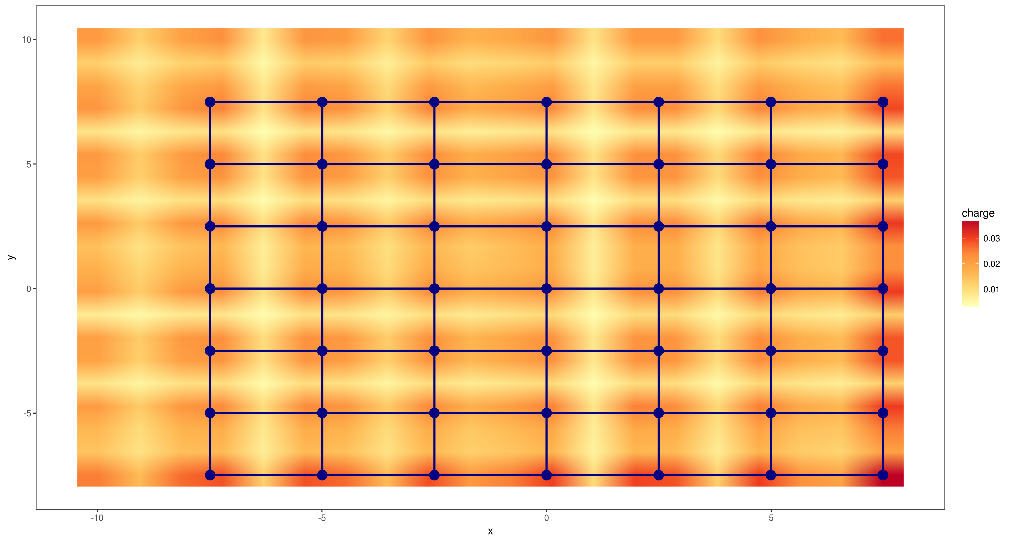
Now we have bonds to the nearest neighbors.
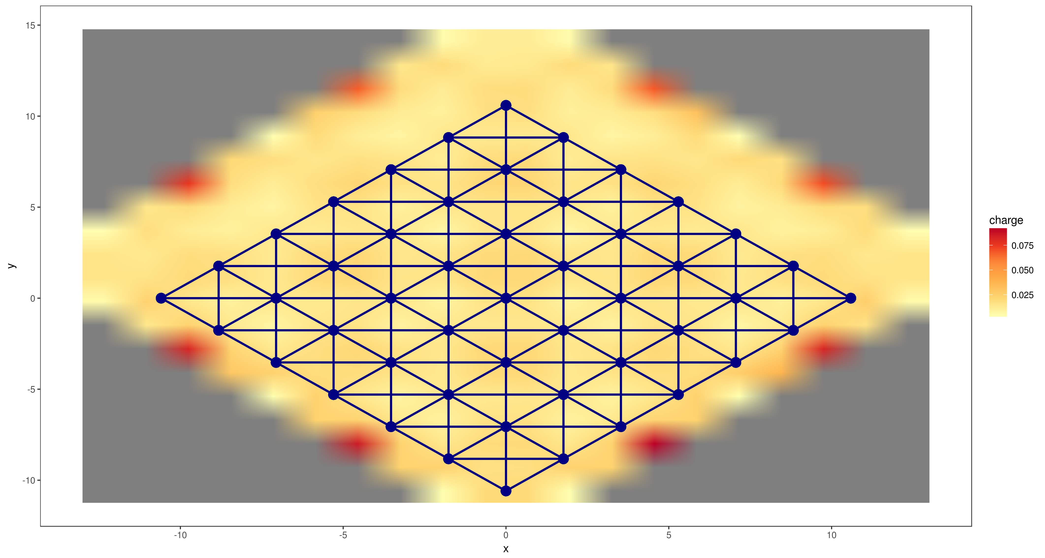
If we want to have additional bonds to the next nearest neighbors we just have to increase the distance argument in the vasp.bonds function. (this time without rotation)
data.plot <- vasp.bonds( data.reproduced, distance = 15 )

vasp.plot( data.plot, 0, 20 ) +
    ## extract just the bonds within the considered plane
    geom_segment( data = data.plot$bonds[
                      data.plot$bonds$z.begin == 0 &
                      data.plot$bonds$z.end == 0, ],
                 aes( x = x.begin, y = y.begin, xend = x.end,
                     yend = y.end ), colour = color.atom, size = 1 )